Simple gene expression
Introduction
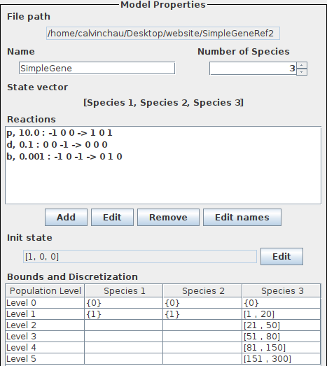
In the following we consider a simple gene expression model. More precisely, we will consider two variations, a slow gene expression and a faster gene expression and demonstrate that our tool is capable of revealing different behaviors. The models can be downloaded here. The reactions of the slow gene expression can be seen below.

Comparison to the classic may abstraction
First, we consider the abstract Markov chain for the gene expression model with population levels {0},[1,20],[21-50],[51-1000] or thresholds 20 and 50 and population bound 1000, respectively.
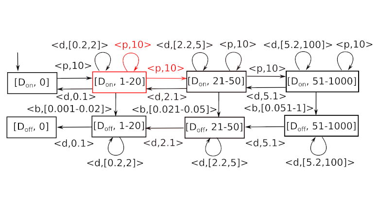
The figure above depicts the classic may abstraction of the transition functions, resulting in non-deterministic self-loops (colored in red). It is practically impossible to conclude anything useful, once we reach such a state. Instead, SeQuaiA considers sequences of transitions and accelerates them. Basically, the self-loops are combined into a transition that brings a typical representative of this population into a lower or higher interval. In this case, the sequences of prevalently growing transitions (those increasing the population) are considered. The resulting abstraction, with the new transition in red, can be seen below. The “A” prefix denotes an accelerated transition.
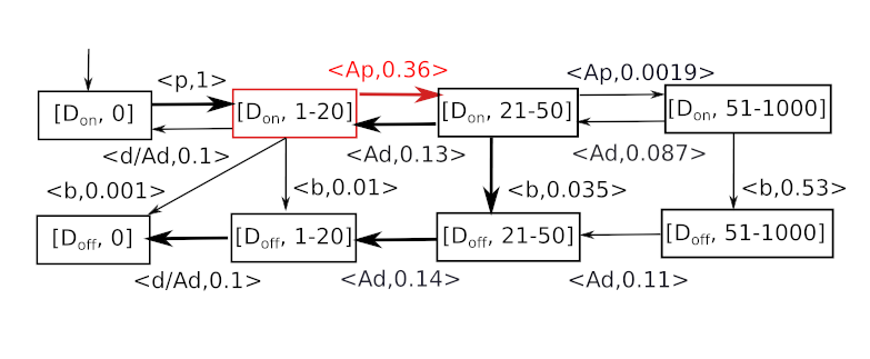
The rate of the accelerated transition reflects the mass-action kinetics with the typical population in the interval and the typical number of transition repetitions before another interval is reached. As can be seen, the abstraction computed by SeQuaiA is easier to analyze and contains significantly less non-determinism.
Slow gene expression
The specification of the slow gene expression in SeQuaiA can be seen below.
We can observe a balanced competition between blocking and oscillation around 70-100 proteins in the simulation shown above.
First, we want to have a look at the full abstraction, which even shows the least probable behaviors. For that, we set the envelope to a large number M, e.g. M=1000000, to include all the behaviors. The result can be seen below.

Indeed, the full abstraction also includes the least probable behaviors and features arbitrary oscillations. We prune the system by choosing a smaller envelope, e.g. envelope = 1 or envelope = 3 and obtain the following results:
envelope = 1

and envelope = 2

Now the abstraction reflects the initial growth, subsequent oscillation only in range of higher populations and blocking and gradual extinction of proteins afterwards.
Fast gene expression
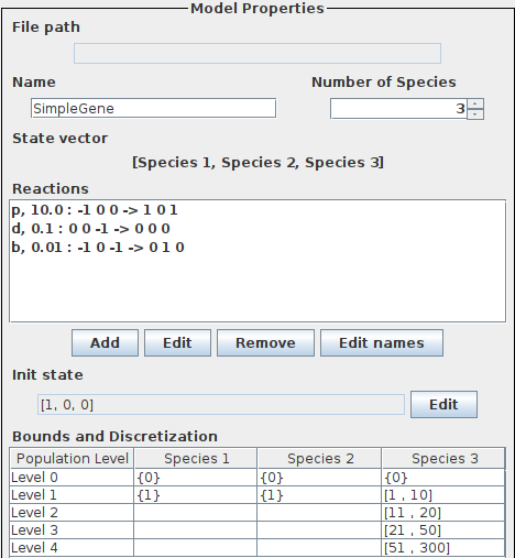
The specification of the fast gene expression in SeQuaiA can be seen below. Compared to the slow gene expression, the blocking rate is higher. As a consequence, the behavior is less complicated.
First, we want to have a look at the full abstraction, which even shows the least probable behaviors. For that, we set the envelope to a large number M, e.g. M=1000000, to include all the behaviors. The result can be seen below.

Indeed, the visualization also includes less probable behaviors, e.g. [1,0,1] -> [0,1,0]. In order to refine our analysis, we decrease the envelope to obtain the most probable behaviors. We set the envelope to 3 and obtain the following visualization:

As can be seen, the new analysis only includes the most probable behaviors. The fast growth until the intervals 2 and 3, but not beyond interval 4, and the slow decline afterwards are revealed. The computed rates induce expected times to pass through a state, matching closely the results of a simulation obtained with the DSD tool (see dotted green line in the figure below). We see that the blocking transition (denoted with b in the specification) has a lower probability (smaller rate) than the production transition (denoted with p in the specification) and thus would not appear in a stricter analysis, e.g. envelope = 2.
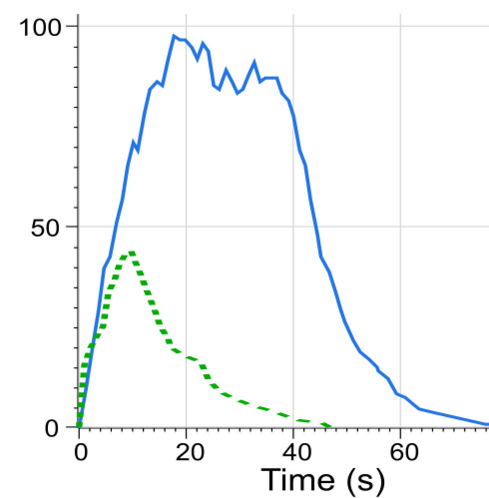
Simulation obtained using the DSD tool
Mean simulation
We consider the slow gene expression model and want to capture the typical behaviors of the system.
The abstraction of the model is shown below (envelope = 2).

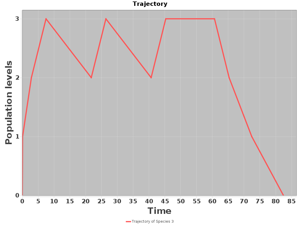
A mean simulation obtained with SeQuaiA is shown below (left). We can observe its validity with respect to the stochastic simulation obtained with the DSD tool (below right, the blue line).

Conclusion
In this example we have seen the differences between the classic may abstraction and SeQuaiA’s abstraction. The latter contains significantly less non-determinism and is therefore easier to analyze. We have demonstrated that our tool is able to reveal different behaviors when a model parameter is changed. Further, the mean simulation is a convenient and fast way to capture the typical behaviors of the system.